Usually the second remarkable limit is written in this form:
\begin(equation) \lim_(x\to\infty)\left(1+\frac(1)(x)\right)^x=e\end(equation)
The number $e$ indicated on the right side of equality (1) is irrational. The approximate value of this number is: $e\approx(2(,)718281828459045)$. If we make the replacement $t=\frac(1)(x)$, then formula (1) can be rewritten as follows:
\begin(equation) \lim_(t\to(0))\biggl(1+t\biggr)^(\frac(1)(t))=e\end(equation)
As with the first remarkable limit, it does not matter which expression stands in place of the variable $x$ in formula (1) or instead of the variable $t$ in formula (2). The main thing is to fulfill two conditions:
- The base of the degree (i.e., the expression in brackets of formulas (1) and (2)) should tend to unity;
- The exponent (i.e. $x$ in formula (1) or $\frac(1)(t)$ in formula (2)) must tend to infinity.
The second remarkable limit is said to reveal the uncertainty of $1^\infty$. Please note that in formula (1) we do not specify which infinity ($+\infty$ or $-\infty$) we are talking about. In any of these cases, formula (1) is correct. In formula (2), the variable $t$ can tend to zero both on the left and on the right.
I note that there are also several useful consequences from the second remarkable limit. Examples of the use of the second remarkable limit, as well as its consequences, are very popular among compilers of standard standard calculations and tests.
Example No. 1
Calculate the limit $\lim_(x\to\infty)\left(\frac(3x+1)(3x-5)\right)^(4x+7)$.
Let us immediately note that the base of the degree (i.e. $\frac(3x+1)(3x-5)$) tends to unity:
$$ \lim_(x\to\infty)\frac(3x+1)(3x-5)=\left|\frac(\infty)(\infty)\right| =\lim_(x\to\infty)\frac(3+\frac(1)(x))(3-\frac(5)(x)) =\frac(3+0)(3-0) = 1. $$
In this case, the exponent (expression $4x+7$) tends to infinity, i.e. $\lim_(x\to\infty)(4x+7)=\infty$.
The base of the degree tends to unity, the exponent tends to infinity, i.e. we are dealing with uncertainty $1^\infty$. Let's apply a formula to reveal this uncertainty. At the base of the power of the formula is the expression $1+\frac(1)(x)$, and in the example we are considering, the base of the power is: $\frac(3x+1)(3x-5)$. Therefore, the first action will be a formal adjustment of the expression $\frac(3x+1)(3x-5)$ to the form $1+\frac(1)(x)$. First, add and subtract one:
$$ \lim_(x\to\infty)\left(\frac(3x+1)(3x-5)\right)^(4x+7) =|1^\infty| =\lim_(x\to\infty)\left(1+\frac(3x+1)(3x-5)-1\right)^(4x+7) $$
Please note that you cannot simply add a unit. If we are forced to add one, then we also need to subtract it so as not to change the value of the entire expression. To continue the solution, we take into account that
$$ \frac(3x+1)(3x-5)-1 =\frac(3x+1)(3x-5)-\frac(3x-5)(3x-5) =\frac(3x+1- 3x+5)(3x-5) =\frac(6)(3x-5). $$
Since $\frac(3x+1)(3x-5)-1=\frac(6)(3x-5)$, then:
$$ \lim_(x\to\infty)\left(1+ \frac(3x+1)(3x-5)-1\right)^(4x+7) =\lim_(x\to\infty)\ left(1+\frac(6)(3x-5)\right)^(4x+7) $$
Let's continue the adjustment. In the expression $1+\frac(1)(x)$ of the formula, the numerator of the fraction is 1, and in our expression $1+\frac(6)(3x-5)$ the numerator is $6$. To get $1$ in the numerator, drop $6$ into the denominator using the following conversion:
$$ 1+\frac(6)(3x-5) =1+\frac(1)(\frac(3x-5)(6)) $$
Thus,
$$ \lim_(x\to\infty)\left(1+\frac(6)(3x-5)\right)^(4x+7) =\lim_(x\to\infty)\left(1+ \frac(1)(\frac(3x-5)(6))\right)^(4x+7) $$
So, the basis of the degree, i.e. $1+\frac(1)(\frac(3x-5)(6))$, adjusted to the form $1+\frac(1)(x)$ required in the formula. Now let's start working with the exponent. Note that in the formula the expressions in the exponents and in the denominator are the same:
This means that in our example, the exponent and the denominator must be brought to the same form. To get the expression $\frac(3x-5)(6)$ in the exponent, we simply multiply the exponent by this fraction. Naturally, to compensate for such a multiplication, you will have to immediately multiply by the reciprocal fraction, i.e. by $\frac(6)(3x-5)$. So we have:
$$ \lim_(x\to\infty)\left(1+\frac(1)(\frac(3x-5)(6))\right)^(4x+7) =\lim_(x\to\ infty)\left(1+\frac(1)(\frac(3x-5)(6))\right)^(\frac(3x-5)(6)\cdot\frac(6)(3x-5 )\cdot(4x+7)) =\lim_(x\to\infty)\left(\left(1+\frac(1)(\frac(3x-5)(6))\right)^(\ frac(3x-5)(6))\right)^(\frac(6\cdot(4x+7))(3x-5)) $$
Let us separately consider the limit of the fraction $\frac(6\cdot(4x+7))(3x-5)$ located in the power:
$$ \lim_(x\to\infty)\frac(6\cdot(4x+7))(3x-5) =\left|\frac(\infty)(\infty)\right| =\lim_(x\to\infty)\frac(6\cdot\left(4+\frac(7)(x)\right))(3-\frac(5)(x)) =6\cdot\ frac(4)(3) =8. $$
Answer: $\lim_(x\to(0))\biggl(\cos(2x)\biggr)^(\frac(1)(\sin^2(3x)))=e^(-\frac(2) (9))$.
Example No. 4
Find the limit $\lim_(x\to+\infty)x\left(\ln(x+1)-\ln(x)\right)$.
Since for $x>0$ we have $\ln(x+1)-\ln(x)=\ln\left(\frac(x+1)(x)\right)$, then:
$$ \lim_(x\to+\infty)x\left(\ln(x+1)-\ln(x)\right) =\lim_(x\to+\infty)\left(x\cdot\ln\ left(\frac(x+1)(x)\right)\right) $$
Expanding the fraction $\frac(x+1)(x)$ into the sum of fractions $\frac(x+1)(x)=1+\frac(1)(x)$ we get:
$$ \lim_(x\to+\infty)\left(x\cdot\ln\left(\frac(x+1)(x)\right)\right) =\lim_(x\to+\infty)\left (x\cdot\ln\left(1+\frac(1)(x)\right)\right) =\lim_(x\to+\infty)\left(\ln\left(\frac(x+1) (x)\right)^x\right) =\ln(e) =1. $$
Answer: $\lim_(x\to+\infty)x\left(\ln(x+1)-\ln(x)\right)=1$.
Example No. 5
Find the limit $\lim_(x\to(2))\biggl(3x-5\biggr)^(\frac(2x)(x^2-4))$.
Since $\lim_(x\to(2))(3x-5)=6-5=1$ and $\lim_(x\to(2))\frac(2x)(x^2-4)= \infty$, then we are dealing with uncertainty of the form $1^\infty$. Detailed explanations are given in example No. 2, but here we will limit ourselves to a brief solution. Making the replacement $t=x-2$, we get:
$$ \lim_(x\to(2))\biggl(3x-5\biggr)^(\frac(2x)(x^2-4)) =\left|\begin(aligned)&t=x-2 ;\;x=t+2\\&t\to(0)\end(aligned)\right| =\lim_(t\to(0))\biggl(1+3t\biggr)^(\frac(2t+4)(t^2+4t))=\\ =\lim_(t\to(0) )\biggl(1+3t\biggr)^(\frac(1)(3t)\cdot 3t\cdot\frac(2t+4)(t^2+4t)) =\lim_(t\to(0) )\left(\biggl(1+3t\biggr)^(\frac(1)(3t))\right)^(\frac(6\cdot(t+2))(t+4)) =e^ 3. $$
You can solve this example in a different way, using the replacement: $t=\frac(1)(x-2)$. Of course, the answer will be the same:
$$ \lim_(x\to(2))\biggl(3x-5\biggr)^(\frac(2x)(x^2-4)) =\left|\begin(aligned)&t=\frac( 1)(x-2);\;x=\frac(2t+1)(t)\\&t\to\infty\end(aligned)\right| =\lim_(t\to\infty)\left(1+\frac(3)(t)\right)^(t\cdot\frac(4t+2)(4t+1))=\\ =\lim_ (t\to\infty)\left(1+\frac(1)(\frac(t)(3))\right)^(\frac(t)(3)\cdot\frac(3)(t) \cdot\frac(t\cdot(4t+2))(4t+1)) =\lim_(t\to\infty)\left(\left(1+\frac(1)(\frac(t)( 3))\right)^(\frac(t)(3))\right)^(\frac(6\cdot(2t+1))(4t+1)) =e^3. $$
Answer: $\lim_(x\to(2))\biggl(3x-5\biggr)^(\frac(2x)(x^2-4))=e^3$.
Example No. 6
Find the limit $\lim_(x\to\infty)\left(\frac(2x^2+3)(2x^2-4)\right)^(3x) $.
Let's find out what the expression $\frac(2x^2+3)(2x^2-4)$ tends to under the condition $x\to\infty$:
$$ \lim_(x\to\infty)\frac(2x^2+3)(2x^2-4) =\left|\frac(\infty)(\infty)\right| =\lim_(x\to\infty)\frac(2+\frac(3)(x^2))(2-\frac(4)(x^2)) =\frac(2+0)(2 -0)=1. $$
Thus, in a given limit we are dealing with an uncertainty of the form $1^\infty$, which we will reveal using the second remarkable limit:
$$ \lim_(x\to\infty)\left(\frac(2x^2+3)(2x^2-4)\right)^(3x) =|1^\infty| =\lim_(x\to\infty)\left(1+\frac(2x^2+3)(2x^2-4)-1\right)^(3x)=\\ =\lim_(x\to \infty)\left(1+\frac(7)(2x^2-4)\right)^(3x) =\lim_(x\to\infty)\left(1+\frac(1)(\frac (2x^2-4)(7))\right)^(3x)=\\ =\lim_(x\to\infty)\left(1+\frac(1)(\frac(2x^2-4 )(7))\right)^(\frac(2x^2-4)(7)\cdot\frac(7)(2x^2-4)\cdot 3x) =\lim_(x\to\infty) \left(\left(1+\frac(1)(\frac(2x^2-4)(7))\right)^(\frac(2x^2-4)(7))\right)^( \frac(21x)(2x^2-4)) =e^0 =1. $$
Answer: $\lim_(x\to\infty)\left(\frac(2x^2+3)(2x^2-4)\right)^(3x)=1$.
|
The first remarkable limit. The derivation of the first remarkable limit is of interest from the point of view of the application of the theory of limits, and therefore we offer you it almost in its entirety. Let's consider the behavior of the function |
 at
at  . To do this, consider a circle of radius 1; let's denote
  .
.Then clearly the area DMOA< площадь сектора МОА < площадьDСОА (см. рис. 1).
S D MOA = 
S MOA =  =
= S D C OA =
Returning to the mentioned inequality and doubling it, we get:
sin x < x < tg x.
After division by term sin x:
 or
or 
Since  , then the variable
  is concluded between two quantities that have the same limit, i.e. , based on the theorem on the limit of the intermediate function of the previous paragraph, we have:
-first wonderful limit .
Example. Calculate the limits of the functions using the first remarkable limit:


Answer. 1) 1, 2) 0, 3)

Exercise: Calculate the limit of a function using the first remarkable limit:

Answer: -2.
The second remarkable limit.
To derive the second remarkable limit, we introduce the definition of the number e:
Definition.
Variable Limit  at
at  called a numbere
:
called a numbere
:
- Second wonderful limit
Number e– irrational number. Its value to ten true decimal places is usually rounded to one true decimal place:
e= 2.7182818284..."2.7.
Theorem. Function  atX
tending to infinity, tending to the limite
:
atX
tending to infinity, tending to the limite
:

Example. Calculate the limits of the functions:

Solution.
According to the properties of limits, the limit of the degree is equal to the degree of the limit, i.e.:


Moreover, in a similar way it can be proven that 


Answer. 1)e 3 , 2)e 2 , 3)e 4 .
Exercise. Calculate the limit of the function using the second remarkable limit:

____________________________________________________________________________________________________________________________________________________________________________________________________________________________________________________________________________________________________________________
ABOUT  answer: e -5
Continuity of a function Continuity of a function at a point
Definition. Functionf ( x ), x Î ( a ; b ) x O Î ( a ; b ), if the limit of the functionf ( x ) at the pointX O exists and is equal to the value of the function at this point:
 .
.
According to this definition, the continuity of the function f(x) at the point X O means the following conditions are met:
function f(x) must be defined at the point X O ;
y function f(x) there must be a limit at the point X O ;
limit of a function f(x) at the point X O must match the value of the function at this point.
Example.
Function f(x)
=
x 2
defined on the entire number line and continuous at a point X= 1 because f( 1)
= 1 and 
Continuity of a function on a set
Definition. Functionf(x), is called continuous on the interval(a; b), if it is continuous at every point of this interval.
If a function is continuous at some point, then this point is called the point of continuity of this function. In cases where the limit of a function at a given point does not exist or its value does not coincide with the value of the function at a given point, then the function is called discontinuous at this point, and the point itself is called a discontinuity point of the function f(x).
Properties of continuous functions.
1) The sum of a finite number of functions continuous at a point A,
2) Product of a finite number of functions continuous at a point A, there is a function that is continuous at this point.
3) The ratio of a finite number of functions continuous at a point A, is a function that is continuous at this point if the value of the function in the denominator is different from zero at the point A.
Example.
Function f(x) = x n, Where n Î N, is continuous on the entire number line. This fact can be proven using property 2 and the continuity of the function f(x) = x.
Function f(x) = sx n (With– constant) is continuous on the entire number line, based on property 2 and example 1.
Theorem 1. A polynomial is a function that is continuous on the entire number line.
Theorem 2 . Any fractional rational function is continuous at every point of its domain of definition.
Example.

Definition
Functionf
(
x
)
called continuous at a pointx = a
, if at this point its increment  tends to zero when the argument increment
  tends to zero, or in other words: functionf
(X)
called continuous at a pointx = a
, if at this point an infinitesimal increment of the argument corresponds to an infinitesimal increment of the function, i.e. if
tends to zero, or in other words: functionf
(X)
called continuous at a pointx = a
, if at this point an infinitesimal increment of the argument corresponds to an infinitesimal increment of the function, i.e. if 
Now, with a calm soul, let’s move on to consider wonderful limits.
looks like .
Instead of the variable x, various functions can be present, the main thing is that they tend to 0.
It is necessary to calculate the limit
As you can see, this limit is very similar to the first wonderful one, but this is not entirely true. In general, if you notice sin in the limit, then you should immediately think about whether it is possible to use the first remarkable limit.
According to our rule No. 1, we substitute zero instead of x:
We get uncertainty.
Now let's try to organize the first wonderful limit ourselves. To do this, let's do a simple combination:
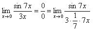
So we organize the numerator and denominator to highlight 7x. Now the familiar remarkable limit has already appeared. It is advisable to highlight it when deciding:
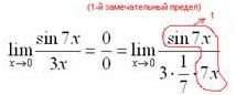
Let's substitute the solution to the first remarkable example and get:
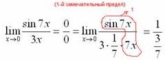
Simplifying the fraction:
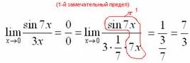
Answer: 7/3.
As you can see, everything is very simple.
Looks like ![]() , where e = 2.718281828... is an irrational number.
, where e = 2.718281828... is an irrational number.
Various functions may be present instead of the variable x, the main thing is that they tend to .
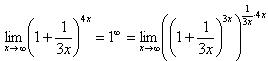
It is necessary to calculate the limit
Here we see the presence of a degree under the sign of a limit, which means it is possible to use a second remarkable limit.
As always, we will use rule No. 1 - substitute x instead of:
It can be seen that at x the base of the degree is , and the exponent is 4x > , i.e. we obtain an uncertainty of the form:
![]()
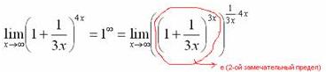
Let's use the second wonderful limit to reveal our uncertainty, but first we need to organize it. As you can see, we need to achieve presence in the indicator, for which we raise the base to the power of 3x, and at the same time to the power of 1/3x, so that the expression does not change:
Don't forget to highlight our wonderful limit:
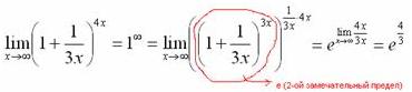
That's what they really are wonderful limits!
If you still have any questions about the first and second wonderful limits, then feel free to ask them in the comments.
We will answer everyone as much as possible.
You can also work with a teacher on this topic.
We are pleased to offer you the services of selecting a qualified tutor in your city. Our partners will quickly select a good teacher for you on favorable terms.
Not enough information? - You can!
You can write math calculations in notepads. It is much more pleasant to write individually in notebooks with a logo (http://www.blocnot.ru).
Formulas, properties and theorems used in solving problems that can be solved using the first remarkable limit are collected. Detailed solutions of examples using the first remarkable limit of its consequences are given.
ContentSee also: Proof of the first remarkable limit and its consequences
Applied formulas, properties and theorems
Here we will look at examples of solutions to problems involving calculating limits that use the first remarkable limit and its consequences.
Listed below are the formulas, properties and theorems that are most often used in this type of calculation.
- The first remarkable limit and its consequences:
. - Trigonometric formulas for sine, cosine, tangent and cotangent:
;
;
;
at , ;
;
;
;
;
;
.
Examples of solutions
Example 1
For this.
1. Calculate the limit.
Since the function is continuous for all x, including at the point, then
.
2. Since the function is not defined (and, therefore, is not continuous) for , we need to make sure that there exists a punctured neighborhood of the point on which . In our case, at . Therefore this condition is met.
3. Calculate the limit. In our case, it is equal to the first remarkable limit:
.
Thus,
.
Similarly, we find the limit of the function in the denominator:
;
at ;
.
And finally, we apply the arithmetic properties of the function limit:
.
Let's apply.
At . From the table of equivalent functions we find:
at ; at .
Then .
Example 2
Find the limit:
.
Solution using the first remarkable limit
At , , . This is the uncertainty of the form 0/0 .
Let's transform the function beyond the limit sign:
.
Let's make a change of variable. Since and for , then
.
Similarly we have:
.
Since the cosine function is continuous on the entire number line, then
.
We apply the arithmetic properties of limits:
.
Solution using equivalent functions
Let us apply the theorem on replacing functions with equivalent ones in the quotient limit.
At . From the table of equivalent functions we find:
at ; at .
Then .
Example 3
Find the limit:
.
Let's substitute the numerator and denominator of the fraction:
;
.
This is the uncertainty of the form 0/0
.
Let's try to solve this example using the first wonderful limit. Since the value of the variable in it tends to zero, we will make a substitution so that the new variable tends not to , but to zero. To do this, we move from x to a new variable t, making the substitution , . Then at , .
We first transform the function beyond the limit sign by multiplying the numerator and denominator of the fraction by:
.
Let's substitute and use the trigonometric formulas given above.
;
;
.
The function is continuous at . We find its limit:
.
Let's transform the second fraction and apply the first wonderful limit:
.
We made a substitution in the numerator of the fraction.
We apply the property of the limit of a product of functions:
.
Example 4
Find the limit:
.
At , , . We have uncertainty of the form 0/0 .
Let's transform the function under the limit sign. Let's apply the formula:
.
Let's substitute:
.
Let's transform the denominator:
.
Then
.
Since and for , we make the substitution and apply the limit theorem complex function and the first remarkable limit:
.
We apply the arithmetic properties of the limit of a function:
.
Example 5
Find the limit of the function:
.
It is easy to see that in this example we have an uncertainty of the form 0/0
. To reveal it, we apply the result of the previous problem, according to which
.
Let us introduce the notation:
(A5.1). Then
(A5.2) .
From (A5.1) we have:
.
Let's substitute it into the original function:
,
Where ,
,
;
;
;
.
We use (A5.2) and the continuity of the cosine function. We apply the arithmetic properties of the limit of a function.
,
here m is a non-zero number, ;
;
;
.
Example 6
Find the limit:
.
When , the numerator and denominator of the fraction tend to 0
. This is the uncertainty of the form 0/0
. To expand it, we transform the numerator of the fraction:
.
Let's apply the formula:
.
Let's substitute:
;
,
Where .
Let's apply the formula:
.
Let's substitute:
;
,
Where .
Numerator of fraction:
.
The function behind the limit sign will take the form:
.
Let's find the limit of the last factor, taking into account its continuity at :
.
Let's apply the trigonometric formula:
.
Let's substitute
. Then
.
Let's divide the numerator and denominator by , apply the first remarkable limit and one of its consequences:
.
Finally we have:
.
Note 1: It was also possible to apply the formula
.
Then .
The formula for the second remarkable limit is lim x → ∞ 1 + 1 x x = e. Another form of writing looks like this: lim x → 0 (1 + x) 1 x = e.
When we talk about the second remarkable limit, we have to deal with uncertainty of the form 1 ∞, i.e. unit in infinite degree.
Let's consider problems in which the ability to calculate the second remarkable limit will be useful.
Example 1
Find the limit lim x → ∞ 1 - 2 x 2 + 1 x 2 + 1 4 .
Solution
Let's substitute the required formula and perform the calculations.
lim x → ∞ 1 - 2 x 2 + 1 x 2 + 1 4 = 1 - 2 ∞ 2 + 1 ∞ 2 + 1 4 = 1 - 0 ∞ = 1 ∞
Our answer turned out to be one to the power of infinity. To determine the solution method, we use the uncertainty table. Let's choose the second remarkable limit and make a change of variables.
t = - x 2 + 1 2 ⇔ x 2 + 1 4 = - t 2
If x → ∞, then t → - ∞.
Let's see what we got after the replacement:
lim x → ∞ 1 - 2 x 2 + 1 x 2 + 1 4 = 1 ∞ = lim x → ∞ 1 + 1 t - 1 2 t = lim t → ∞ 1 + 1 t t - 1 2 = e - 1 2
Answer: lim x → ∞ 1 - 2 x 2 + 1 x 2 + 1 4 = e - 1 2 .
Example 2
Calculate the limit lim x → ∞ x - 1 x + 1 x .
Solution
Let's substitute infinity and get the following.
lim x → ∞ x - 1 x + 1 x = lim x → ∞ 1 - 1 x 1 + 1 x x = 1 - 0 1 + 0 ∞ = 1 ∞
In the answer, we again got the same thing as in the previous problem, therefore, we can again use the second wonderful limit. Next we need to select at the base power function whole part:
x - 1 x + 1 = x + 1 - 2 x + 1 = x + 1 x + 1 - 2 x + 1 = 1 - 2 x + 1
After this, the limit takes the following form:
lim x → ∞ x - 1 x + 1 x = 1 ∞ = lim x → ∞ 1 - 2 x + 1 x
Replace variables. Let's assume that t = - x + 1 2 ⇒ 2 t = - x - 1 ⇒ x = - 2 t - 1 ; if x → ∞, then t → ∞.
After that, we write down what we got in the original limit:
lim x → ∞ x - 1 x + 1 x = 1 ∞ = lim x → ∞ 1 - 2 x + 1 x = lim x → ∞ 1 + 1 t - 2 t - 1 = = lim x → ∞ 1 + 1 t - 2 t 1 + 1 t - 1 = lim x → ∞ 1 + 1 t - 2 t lim x → ∞ 1 + 1 t - 1 = = lim x → ∞ 1 + 1 t t - 2 1 + 1 ∞ = e - 2 · (1 + 0) - 1 = e - 2
To perform this transformation, we used the basic properties of limits and powers.
Answer: lim x → ∞ x - 1 x + 1 x = e - 2 .
Example 3
Calculate the limit lim x → ∞ x 3 + 1 x 3 + 2 x 2 - 1 3 x 4 2 x 3 - 5 .
Solution
lim x → ∞ x 3 + 1 x 3 + 2 x 2 - 1 3 x 4 2 x 3 - 5 = lim x → ∞ 1 + 1 x 3 1 + 2 x - 1 x 3 3 2 x - 5 x 4 = = 1 + 0 1 + 0 - 0 3 0 - 0 = 1 ∞
After that, we need to transform the function to apply the second great limit. We got the following:
lim x → ∞ x 3 + 1 x 3 + 2 x 2 - 1 3 x 4 2 x 3 - 5 = 1 ∞ = lim x → ∞ x 3 - 2 x 2 - 1 - 2 x 2 + 2 x 3 + 2 x 2 - 1 3 x 4 2 x 3 - 5 = = lim x → ∞ 1 + - 2 x 2 + 2 x 3 + 2 x 2 - 1 3 x 4 2 x 3 - 5
lim x → ∞ 1 + - 2 x 2 + 2 x 3 + 2 x 2 - 1 3 x 4 2 x 3 - 5 = lim x → ∞ 1 + - 2 x 2 + 2 x 3 + 2 x 2 - 1 x 3 + 2 x 2 - 1 - 2 x 2 + 2 - 2 x 2 + 2 x 3 + 2 x 2 - 1 3 x 4 2 x 3 - 5 = = lim x → ∞ 1 + - 2 x 2 + 2 x 3 + 2 x 2 - 1 x 3 + 2 x 2 - 1 - 2 x 2 + 2 - 2 x 2 + 2 x 3 + 2 x 2 - 1 3 x 4 2 x 3 - 5
Since we now have the same exponents in the numerator and denominator of the fraction (equal to six), the limit of the fraction at infinity will be equal to the ratio of these coefficients at higher powers.
lim x → ∞ 1 + - 2 x 2 + 2 x 3 + 2 x 2 - 1 x 3 + 2 x 2 - 1 - 2 x 2 + 2 - 2 x 2 + 2 x 3 + 2 x 2 - 1 3 x 4 2 x 3 - 5 = = lim x → ∞ 1 + - 2 x 2 + 2 x 3 + 2 x 2 - 1 x 3 + 2 x 2 - 1 - 2 x 2 + 2 - 6 2 = lim x → ∞ 1 + - 2 x 2 + 2 x 3 + 2 x 2 - 1 x 3 + 2 x 2 - 1 - 2 x 2 + 2 - 3
By substituting t = x 2 + 2 x 2 - 1 - 2 x 2 + 2 we get a second remarkable limit. This means that:
lim x → ∞ 1 + - 2 x 2 + 2 x 3 + 2 x 2 - 1 x 3 + 2 x 2 - 1 - 2 x 2 + 2 - 3 = lim x → ∞ 1 + 1 t t - 3 = e - 3
Answer: lim x → ∞ x 3 + 1 x 3 + 2 x 2 - 1 3 x 4 2 x 3 - 5 = e - 3 .
Conclusions
Uncertainty 1 ∞, i.e. unity to an infinite power is a power-law uncertainty, therefore, it can be revealed using the rules for finding the limits of exponential power functions.
If you notice an error in the text, please highlight it and press Ctrl+Enter